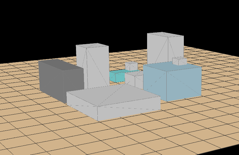
PyQtGraph: Box scenery

This post is about creating something like...

...using pyqtgraph.

Why?

Because of a project involving solar-thermal panels, at the beginning of this year, I realized that the way of obtaining how much shadow-per-year-percentage an object projects over another object was very inaccurate. So I attempted  to create a sun-simulator, where you place the objects that are near to the place you want to study and then, run a script that draws shadows (with their grey color as a function of the % of shadow) over the place. That way, you can smartly place your solar collector.

I've not gone that further, I left the (short) development once I knew that something ~ similar existed for free. Don't reinvent the wheel.

But I want to show this, because maybe it helps you to go a step forward with your own project.

The code is posted here (there are comments explaining how to create "buildings" and "panels")

If you have pyqtgraph in your system, copy and paste the code in a python terminal and you should see something.

I've been playing today with the camera positions, with the remote idea of a video-game in mind.

Camera command (I haven't found this at pyqtgraph docs, but here) example:

WINDOWOBJECT.setCameraPosition(distance=100,elevation=10,azimuth=30)



Greetings, Javier

3D Mechanism Animation with PyQtGraph

In a study break I have coded an animated 3d mechanism. Is very simple in order to get it working quickly, but shows the basics of 3d plots with pyqtgraph.

Screenshot:

Code:

from pyqtgraph.Qt import QtCore, QtGui

import pyqtgraph.opengl as gl

import pyqtgraph as pg

import numpy as np

app = QtGui.QApplication([])

w = gl.GLViewWidget()

w.opts['distance'] = 40

w.show()

w.setWindowTitle('3d wire crankshaft')

i=0

crankshaft=np.array(([0,0,0],[2,0,0],[2,np.cos(i),np.sin(i)],[2.5,np.cos(i),np.sin(i)],[2.5,-np.cos(i),-np.sin(i)],[3,-np.cos(i),-np.sin(i)],[3,0,0],[6,0,0]))

plt=gl.GLLinePlotItem(pos=crankshaft)

w.addItem(plt)

conrod1=np.array(([2.25,np.cos(i),np.sin(i)],[2.25,np.cos(i)+2.5,0]))

plt1=gl.GLLinePlotItem(pos=conrod1)

w.addItem(plt1)

conrod2=np.array(([3.25,-np.cos(i),-np.sin(i)],[3.25,-np.cos(i)-2.5,0]))

plt2=gl.GLLinePlotItem(pos=conrod2)

w.addItem(plt2)

def crankshaft():

  global i

  crankshaft=np.array(([0,0,0],[2,0,0],[2,np.cos(i),np.sin(i)],[2.5,np.cos(i),np.sin(i)],[2.5,-np.cos(i),-np.sin(i)],[3,-np.cos(i),-np.sin(i)],[3,0,0],[6,0,0]))

  conrod1=np.array(([2.25,np.cos(i),np.sin(i)],[2.25,np.cos(i)+2.5,0]))

  conrod2=np.array(([2.75,-np.cos(i),-np.sin(i)],[2.75,-np.cos(i)-2.5,0]))

  plt.setData(pos=crankshaft)

  plt1.setData(pos=conrod1)

  plt2.setData(pos=conrod2)

  i+=0.05

time=QtCore.QTimer()

time.timeout.connect(crankshaft)

time.start(0.1) 

This time I'm not explaining line by line because I think is easy to see what is happening. 

Any doubts, comment. 

Bye!

Typical degree problem & Python: Part 3

Problem 3 formulation:

Given a line described by ax+by+c=0, create a function script with the values a,b,c as input that prints:

1-The affine transformation matrix obtained by creating a symmetry respect to the line

2-A plot of a circle with 1 unit radius centered on (0,0) and its reflection

Solution:

##### Libraries #####

from numpy import *

import math as mt # Mistake corrected

import pyqtgraph as pg

pg.setConfigOption('background','w') # Changes plot window background to white

####################

def tafin(a,b,c):       # function declaration

  window=pg.plot(title="Reflection") # Creates plot window called window

  Ax=linspace(-5,5)    # Generates values from -5 to 5

  Ay=-a*Ax/b-c/b       # Line equation

  window.plot(Ax,Ay)       # Plots line

  alpha=linspace(0,2*pi) # Generates alpha values

  Bx=cos(alpha)          # X coordinates of the (0,0) centered circumference 

  By=sin(alpha)          # Y coordinates of the (0,0) centered circumference 

  window.plot(Bx,By,pen='r') # Plots (0,0) centered circumference in red colour

  B1s=ones((1,size(Bx)))        # Line vector filled with 1's

  F=vstack((Bx,By,B1s)) # Compounds an array from Bx,By and B1s

  XA=0     # random point

  YA=(-a/b)*XA-(c/b)     # Obtains one point of the symetry line

  XB=1     # another random point

  YB=(-a/b)*XB-(c/b)     # Obtains another point of the symetry line

  # Symetry matrix

  Ta1=array(([XA,XB,-a],[YA,YB,-b],[1,1,0])) # Mirrored points coincident with line

  Ta2=linalg.inv(array(([XA,XB,a],[YA,YB,b],[1,1,0])))  # Original line coincident points

  Ta=dot(Ta1,Ta2) # Symetry matrix

  S=dot(Ta,F)     # Mirrors the circumference coordinates stored in F

  window.plot(S[0,:],S[1,:],pen='b') # Plots mirrored circumference in blue

  print "The affine transformation matix is"  #

  print Ta   # prints affine transformation matrix 

Open a terminal, paste the function and then type something like tafin(2.0,1.0,4.0)  the output should be very similar to the screenshot. 

Solving this problem with python has allowed me to understand more things about this language, for example, I used to import math as * alongside with numpy as *, this should not be done. The first thing where you can see how that affects to coding is the absence of "for" bucles to operate within arrays and their elements. 

This clearly makes the code easier, cleaner and more efficient and shorter than the matlab equivalent.

The new thing with the pyqtgraph module are the color plots, and plot background, easy to perform. 

With this problem I finish this little section about algebra and python, hope that you got something good from it. 

Bye!

Typical degree problem & Python: Part 2

Problem 2 formulation:

Create a script that plots an n vertexes polygon inscribed in an ellipse with semi axis a=7, b=2. Solve for n=12

Solution:

##### Libraries #####

from numpy import *

import pyqtgraph as pg

#####################

a=7 # Semi axis X value

b=2 # Semi axis Y value 

n=12 # Polygon vertex number

window=pg.plot(title="Inscribed Polygon") #Creates plot window called window

alpha=linspace(0,2*pi) # Creates line matrix with values from 0 to 2*pi

SA=size(alpha) # Gets the size of alpha matrix

E=zeros([2,SA]) # Creates a 2xSA matrix filled with zeros

for i in range(SA): # Gets X,Y values of the ellipse and stores them in E[0,i]
  E[0,i]=a*cos(alpha[i])
  E[1,i]=b*sin(alpha[i])

window.plot(E[0,:],E[1,:]) # Plots the ellipse

V=zeros([2,n+1]) # Array filled with zeros that will contain polygon vertexes
alpha=0 # Variable reset

for i in range (n+1): # Bucle that obtains the coordinates of an n vertexes polygon
  V[0,i]=cos(alpha)
  V[1,i]=sin(alpha)
  alpha+=2*pi/n

VSM=[[a,0],[0,b]] # Transformation matrix that will inscribe the polygon inside the ellipse

V=dot(VSM,V) # Transformation matrix * Polygon

window.plot(V[0,:],V[1,:]) # Plots the polygon




To see it working, open a terminal (ctrl+alt+t), type "python" and then copy-paste the code.(you need to have installed the pyqtgraph module in order to plot, see this post)

This problem is very similar to the Problem 1 and without the importing part it is almost equal to the matlab script.


Next post will be about mirroring an image with a line equation as a mirror line. 

Stay tuned, bye!

Typical degree problem & Python: Part 1

Recently I've been forced to use Matlab for solving some algebra exercises for my degree.
Matlab drives me mad in several ways and even before typing the first line of code, I've been thinking about solving the problems with python.

Let's start.

Problem 1 formulation:

Draw an ellipse with its semi axes measuring a=5 and b=2, then create a script that plots a number n of ellipses equal in size with common center, solve for n=30. Each ellipse should be rotated an angle of pi/n radian from the previous one. The output of the script should look like this:

Solution:

##### Libraries #####

from numpy import *

from math import *

import pyqtgraph as pg

#####################

##### Input Variables

a=7  # semi axis X value

b=2  # semi axis Y value

n=30 # number of ellipses

#####################

window=pg.plot(title="Concentric Ellipses") #Creates plot window called window

alpha=linspace(0,2*pi) # Creates line matrix with values from 0 to 2*pi

SA=size(alpha) # Gets the size of alpha matrix

E=zeros([2,SA]) # Creates a 2xSA matrix filled with zeros

for i in range(SA): # Gets X,Y values of the ellipse and stores them in E
  E[0,i]=a*cos(alpha[i])
  E[1,i]=b*sin(alpha[i])

beta=0 # Ellipse angle variable inicialization

for i in range(n): # Generates n concentric ellipses angled pi/n radians 
  
  TM=[[cos(beta),-sin(beta)],[sin(beta),cos(beta)]] # Transformation matrix
     
  RE=dot(TM,E) # RE contains the coordinates of the rotated ellipse
  
  REX=RE[0,:] # RE X values extraction
  REY=RE[1,:] # RE Y values extraction
  
  window.plot(REX,REY) # Plots the current rotated ellipse
  
  beta+=pi/n # Increases beta by pi/n steps
  


To see it working, open a terminal (ctrl+alt+t), type "python" and then copy-paste the code.
(you need to have installed the pyqtgraph module in order to plot, see this post)

The main difference between python and matlab scripts for this exercise is the library import header, being the rest of them very mimetic.


Second exercise on the next post, bye!

Mechanism animation with PyQtGraph

Linux isn't only FreeCAD.

I have always wanted to create animated mechanisms using python and a plot library. Not only the mechanisms, but a small program that could be used without typing a word of code at all (a personal project).

I found matplotlib very similar to matlab, but not very well suited to create a graphical interface with it. 

But yesterday I tried PyQtGraph and was amazed with how easy is to create dialog boxes and very complex plots, plus people says is faster than matplotlib. 

The con has been a step learning curve.

The install was easy downloading the deb package from the site and using gdebi. I did not need anything extra to get it working.

Slider-Crank Mechanism

Once installed PyQtGraph, open a terminal (ctrl+alt+t) and type "python" (without quotes), then copy-paste this code:

import math
import pyqtgraph as pg
from pyqtgraph.Qt import QtCore, QtGui

window=pg.plot(title="Crank-Slider Mechanism")

i=0
def update():  
  global i
  x1=[0,math.cos(i),2+math.cos(i)]
  y1=[0,math.sin(i),0]
  
  if(i<360):
    i+=0.003
  else:
    i=0
    
  window.plot(x1,y1,clear=True)

time=QtCore.QTimer()
time.timeout.connect(update)
time.start(0.1) 

  

A window like this should appear in your screen with a slider-crank mechanism moving inside.

Step by Step

To create a plot window:

window=pg.plot(title="Crank-Slider Mechanism")

"window" is the variable where we save the plot window, pg is the name we give to the imported pyqtgraph library and the part inside brackets gives name to the plot window.

The function "update()" plots the mechanism advancing one step every time is called. The crank angle (i) is increased until it reaches 360º, then i resets to 0.

x1 and y1 are x and y point values at every step. This is no the "formal" way of doing this things, but is easy and fast.  If someone wants to dig more, crank is 1 unit long and crank to slider bar is 2 units long.

window.plot(x1,y1,clear=True)

It plots x,y data inside "window" and with the parameter "clear" it erases previous plot before plotting the new one.

The timer events is the most obscure part of the script, what I think it does is:

time=QtCore.QTimer()  # Creates a timer

time.timeout.connect(update) # Executes a function when time is up

time.start(0.1) # Starts timer and counts to 0.1 milliseconds

And this is all I have learnt of pyqtgraph at the moment, next step could be something like dialog boxes that modify bar dimensions.  

Hope you could see the mechanism moving, if not, comment something. (If you liked it, you can comment too ;) )

bye!

Bearings from scripted sketches

Hi all, I'm back. I have been very busy with my college but now I have a little time to play with this things again.

Let's script!

Latest thing i did was about increasing the speed of the bearing generator macro. I realized that any boolean involving a torus will spend a lot of time to generate.

Torus is needed to create the groove of the ball bearing and the only way I've imagined to do something similar without using torus was creating the bearing ring profile and revolving.

This is what I am going to explain in this post, how to create bearings using scripted sketches.

Note: full code at the bottom

This picture should explain easily how we want to achieve that:

Area A equals to the profile of the outter ring, area B to the profile of the inner ring and C is the groove of the bearing. 

A and B rectangles have they edges opened because we want to round them (once we are sketching, is just easier this way than using booleans for rounding corners). This rounding is accomplished by arcs.

I'm explaining only one ring with detail, inner and outter ring are actually the same process (copy-paste)

First of all, libraries needed:

import Part
import math
from FreeCAD import Base

Profile definition: Lines and Arcs

To introduce a line object from A to B in FreeCAD by command line type:

LineName=Part.makeLine((AX,AY,AZ),(BX,BY,BZ))


To create an arc object with radius, center position, orientation and angle, do:

ArcName=Part.makeCircle(Radius, Base.Vector(CenterX,CenterY,CenterZ), BaseVector(DirectionX,DirectionY,DirectionZ), StartingAngle, EndingAngle)


The vector BaseVector(DirectionX,DirectionY,DirectionZ)  must be perpendicular to the plane where we want the arc to be placed.
For example, if we ant the arc to be in a XY plane, one perpendicular vector would be (0,0,1).

Starting angle and ending angle provides the ability to create arcs and is also dependent of the plane where we have placed the arc.  This is harder to explain but anyone wanting to go further just read a bit about cross product

For what we are doing here, our direction is (0,0,1) which makes starting and ending angles to be specified in the normal counter-clockwise format.

Now take some time to obtain the points A to B of every line (z always 0):

A means starting point.
B means ending point.

Line 1 (L1):

L1 A X position= r1
L1 A Y position= Radial thickness

L1 B X position= Bearing thickness - r1
L1 B Y position= Radial thickness

L1 command:

L1=Part.makeLine((r1, Radial thickness, 0), (Bearing thickness - r1, Radial thickness, 0))

Line 2 (L2):

L2 A X position=Bearing thickness
L2 A Y position=Radial thickness - r1

L2 B X position=Bearing thickness
L2 B Y position=r2

L2 command:

L2=Part.makeLine((Bearing thickness, Radial thickness - r1), (Bearing thickness, r2))


This is more tedious than complicated, I think is easy to continue and create the 2 lines left. If you have problems, please, comment.


Arc

Arc is more less the same but has an extra feature that is the starting and ending point.

To create the upper left arc:

Center position:

X=r1
Y=Radial thickness - r1
Z=0

Angle:

Start angle*=90º
End angle*=180º

*using vector (0,0,1) as arc placement

Arc command:

A1=Part.makeCircle(r1, Base.Vector(r1, Radialthickness - r1, 0), Base.Vector(0,0,1), 90, 180)


Upper right arc:

Center position:

X=Bearing thickness - r1
Y=Radial thickness - r1
Z=0

Angle:

Start angle*=0º
End angle*=90º

*using vector (0,0,1) as arc placement

Arc command:

A1=Part.makeCircle(r1, Base.Vector(Bearing thickness - r1, Radialthickness - r1, 0), Base.Vector(0,0,1), 0, 90)


The same as lines, I think is easy to create the two arc remaining.


Now we have arcs and lines that aren't nothing more by themselves. To link everything together, we create a wire.

Wire command is easy:

Wiredthing=Part.Wire( [ thingA, thingB, thingC, ... , thing N ] )


If you followed my naming method, your wire command should be something like:

ProfileWire=Part.Wire( [L1,A1,L2,A2,L3,A3,L4,A4] )


From wire we can create a face by typing:

ProfileFace=Part.Face(ProfileWire)


If you give some value to Radial thickness and Bearing thickness, this should be the output of the whole thing above (remember Part.show(NAME) to make it visible):

You can see here the orientation:

Faces can be involved in boolean operations and to create the groove of the bearing, we are going to cut our surface with a circle.

To create a circle:

Circle=Part.makeCircle(CircleRadius, Base.Vector(0,0,0), Base.Vector(0,0,1),0, 360)

Circle=Part.Wire([Circle])

Circle=Part.Face(Circle)

Part.show(Circle)

Positioning and cutting: 

This is exactly the same that has been used in previous scripts. 

To move something just:

TraslationVector(X, Y, Z)

Something.translate(TranslationVector)

To cut two parts:

CuttedPart=PartA.cut(PartB)

Where par B cuts partA.


Be careful when moving our ring section because the translation vector will position the parte from the relative zero where it was created.
The circle relative zero is positioned on its center.


At the end we should se something like this (depending where you have moved your circle you will see something different or nothing at all if both surfaces do not intersect):

The outer ring profile is done with this steps. Inner ring is almost equal, if you have problems after reading the full code, comment.

Revolving faces

With the profile defined and ready, we can go from 2d to 3d by revolving the face. 

Command:

RevolutedFace=Face.revolve(Base.Vector(0,0,0), Base.Vector(360,0,0))

First Base.Vector has something to do about axis scale, we do not want to distort our face so just keep it (0,0,0). Second Base.Vector tells the rev axis and how many degrees of revolution we want. 360 means full revolution.

Screenshot:

Few milliseconds and we have the outer ring, with groove and rounded corners. This could take up to 4-5 seconds when using the torus method. 

Using the same method to the inner ring and adapting the ball generator from previous scripts, we have a bearing like this one:

Not too different from previous versions, but faster to load. 

Plus this method gives me the ability to create new types of bearings with increased complexity, like conical thrust bearing. 

CODE

This code, as is, will generate the above bearing and any other you need only changing the input parameters.

#############################################################

#######  JMG December 2013 Linux Mint 15 KDE  ###############

#############################################################

import Part

import math

from FreeCAD import Base

################  INPUT PARAMETERS  #####################

rout=20             ###External radius

rin=10              ###Inner radius

bth=8               ###Bearing thickness

##########################################

DeltaR=rout-rin

Lb=((rout-rin)/2)+rin

Rb=0.3*bth

##############  Outer ring (a)  ##############################:

r1a=1

r2a=0.5

btha=bth                  ###UPPER RING THICKNESS

rtha=rout-Lb-0.8*Rb       ###UPPER RING RADIAL THICKNESS

#Lines

L1a=Part.makeLine((r1a,rtha,0),(btha-r1a,rtha,0))

L2a=Part.makeLine((btha,rtha-r1a,0),(btha,r2a,0))

L3a=Part.makeLine((btha-r2a,0,0),(r2a,0,0))

L4a=Part.makeLine((0,r2a,0),(0,rtha-r1a,0))

#Corner rounding

A1a=Part.makeCircle(r1a,Base.Vector(btha-r1a,rtha-r1a,0),Base.Vector(0,0,1),0,90)

A2a=Part.makeCircle(r2a,Base.Vector(btha-r2a,r2a,0),Base.Vector(0,0,1),270,360)

A3a=Part.makeCircle(r2a,Base.Vector(r2a,r2a,0),Base.Vector(0,0,1),180,270)

A4a=Part.makeCircle(r1a,Base.Vector(r1a,rtha-r1a,0),Base.Vector(0,0,1),90,180)

##################

Ur=Part.Wire([L1a,A1a,L2a,A2a,L3a,A3a,L4a,A4a])

Ur=Part.Face(Ur)

VUR=(0,rout-rtha,0)

Ur.translate(VUR)

################Inner ring(b):################################:

r1b=0.5

r2b=0.5

bthb=bth

rthb=rtha

#Lines

L1b=Part.makeLine((r1b,rthb,0),(bthb-r1b,rthb,0))

L2b=Part.makeLine((bthb,rthb-r1b,0),(bthb,r2b,0))

L3b=Part.makeLine((bthb-r2b,0,0),(r2b,0,0))

L4b=Part.makeLine((0,r2b,0),(0,rthb-r1b,0))

#Corner rounding

A1b=Part.makeCircle(r1b,Base.Vector(bthb-r1b,rthb-r1b,0),Base.Vector(0,0,1),0,90)

A2b=Part.makeCircle(r2b,Base.Vector(bthb-r2b,r2b,0),Base.Vector(0,0,1),270,360)

A3b=Part.makeCircle(r2b,Base.Vector(r2b,r2b,0),Base.Vector(0,0,1),180,270)

A4b=Part.makeCircle(r1b,Base.Vector(r1b,rthb-r1b,0),Base.Vector(0,0,1),90,180)

###########################################################

Ir=Part.Wire([L1b,A1b,L2b,A2b,L3b,A3b,L4b,A4b])

Ir=Part.Face(Ir)

VIR=(0,rin,0)

Ir.translate(VIR)

####################  GROOVE  #############################

Rb=0.25*(rout-rin)

  

groove=Part.makeCircle(Rb,Base.Vector(0,0,0),Base.Vector(0,0,1),0,360)

  

groove=Part.Wire([groove])

  

groove=Part.Face(groove)

VGROOVE=(bth/2,Lb,0)

groove.translate(VGROOVE)

  

#Cut

  

Ur=Ur.cut(groove)

Ir=Ir.cut(groove)

######################## 3D ############################

Ur=Ur.revolve(Base.Vector(0,0,0),Base.Vector(360,0,0))

Ir=Ir.revolve(Base.Vector(0,0,0),Base.Vector(360,0,0))

################### Ball Creator ########################

BN=(math.pi*Lb)*0.8/(Rb)   ### BALL NUMBER

BN=math.floor(BN)

BN=int(BN)

for i in range (BN):

 Sph=Part.makeSphere(Rb)

 Alpha=(i*2*math.pi)/BN

 VSph=(bth/2, Lb*math.sin(Alpha), Lb*math.cos(Alpha))

 Sph.translate(VSph)

 Part.show(Sph)

### Show parts

Part.show(Ur)

Part.show(Ir)

I want to create more scripted parts this holidays, stay tuned.

Bye!